Welcome to the Research Platform. This guide is designed to get you up and running as quickly as possible by walking through a typical first day on the system—from launching your first machine to securely saving your work and shutting down.

Before You Start

To log in, you must already be a member of an active project and have either:

• A standard NASA identity, OR
• A STAR ID (for external partners).

(Don't have these yet? See How to get access.)

Quick Summary

The rest of this page walks through your first day on the platform step-by-step. If you just want the essentials, here is the one-minute version to get you moving immediately.

1. Go to rp.sciencecloud.nasa.gov and log in.
2. Pick a machine size. Start it.
3. Keep files in ~, in /efs/<project>, or in object storage. Everything else is lost on restart.
4. Work in a notebook. Ask the SI assistant when you are stuck. Need your own packages? Build a conda environment in ~/envs and register it as a kernel.
5. Big job? Dask for parallel work, NBQueue for long background runs.
6. Same file as a colleague? Use the collaboration tile.
7. Check the usage panel.
8. Stop everything when you finish.

Getting Started: Step-by-Step

Step 1: Log In

1. Open rp.sciencecloud.nasa.gov in your web browser.
2. Sign in. You will be briefly redirected to the Science Cloud login service (STAR) to verify your identity.
3. Once signed in, you will land on the platform's main launch screen. There is nothing to install.

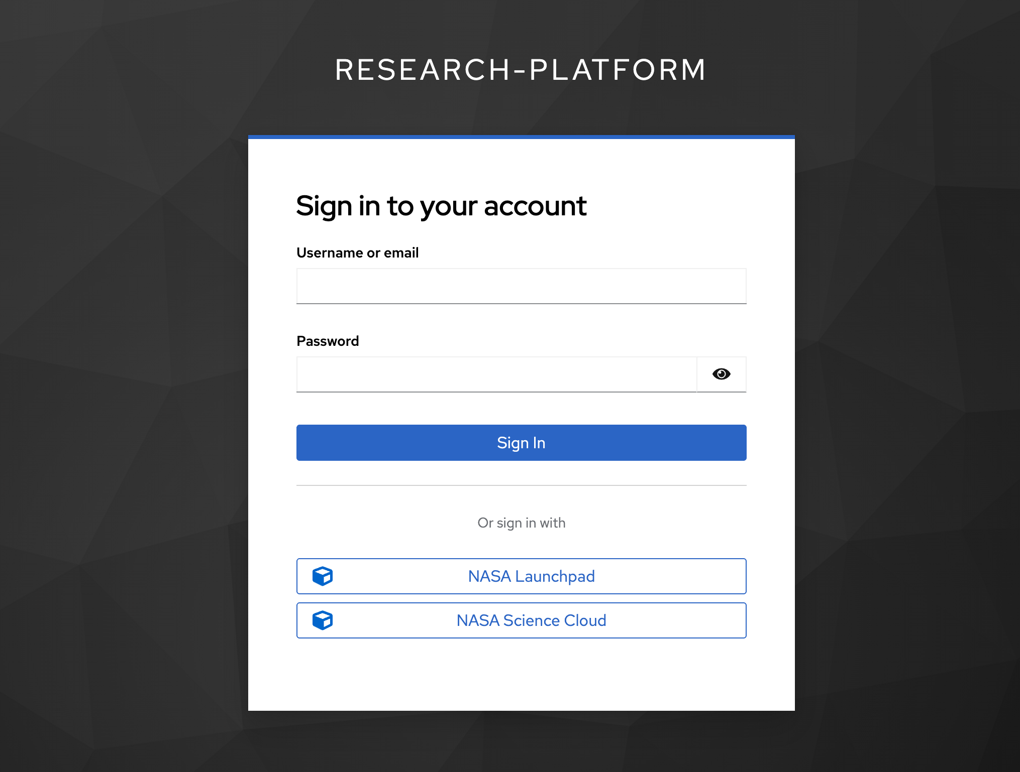
The sign-in page. Use your NASA Launchpad or NASA Science Cloud identity.

Step 2: Choose Your Settings and Start

1. Once logged in, you will land on the Server Options screen. You need to make three choices here before starting your workspace:

How big of a machine do you need? Choose your compute power from the Server Type dropdown list:

Coming later: Two changes to this list are on the roadmap: adding GPU machines, and letting project admins build and maintain their own custom list of server types for their team, instead of everyone choosing from one platform-wide list.

Which software stack do you need? Select a ready-made science stack from the Images dropdown list. (An image is a packaged set of software, for example, Earth Science Server with SI Intelligence). (Note: If your project uses a custom container image, you can enter it into the "Other image" box).

Which project are you working on? Select your active project from the Project dropdown list. This determines which project storage you can access and which budget will be charged for this session.

1. Once you have made your selections, click Start. Your workspace will open in a minute or two.

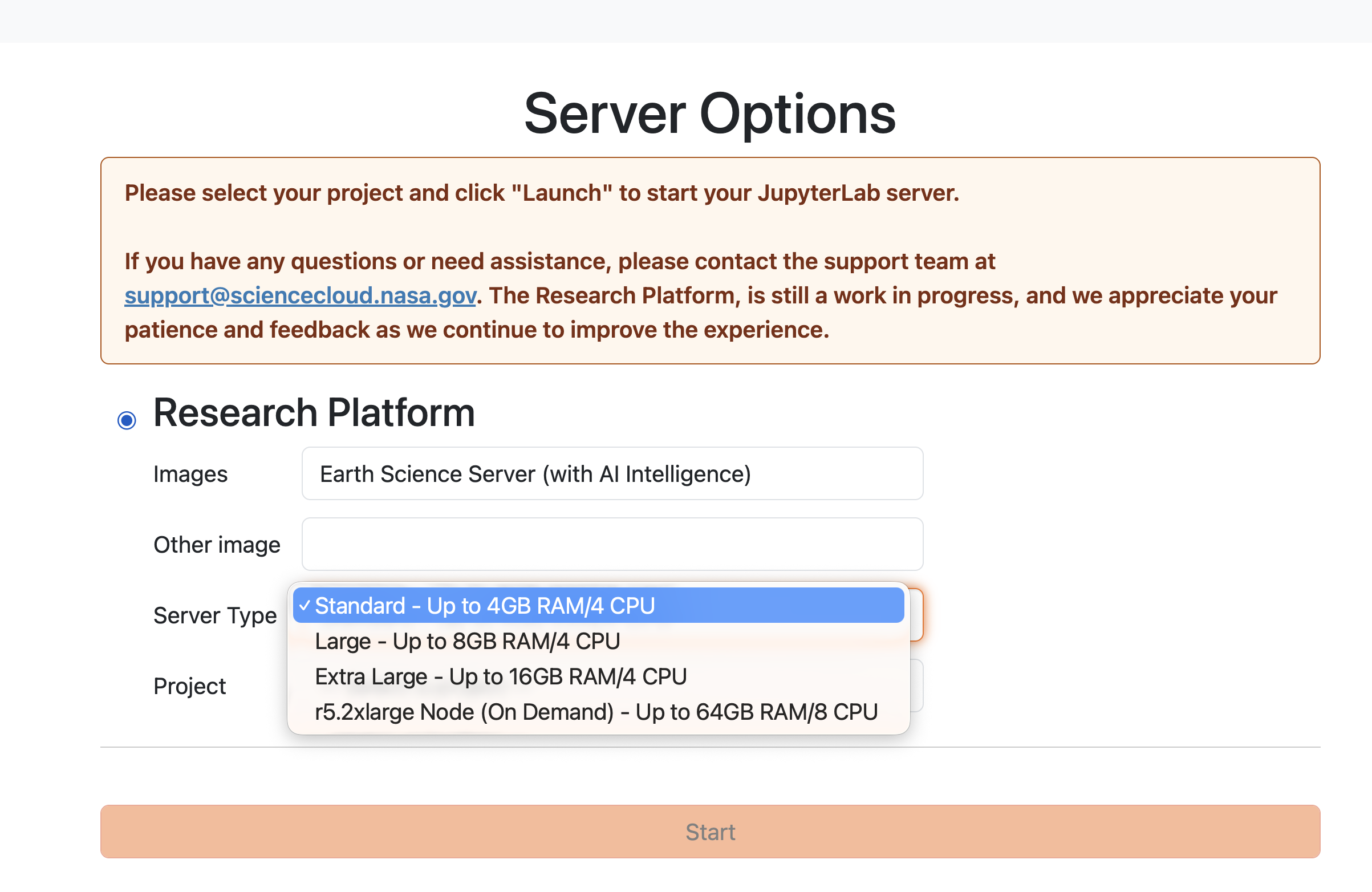
The Server Options screen: pick the image, the server type, and the project.

Step 3: Find Your Way Around JupyterLab

You are now in JupyterLab. The important parts:

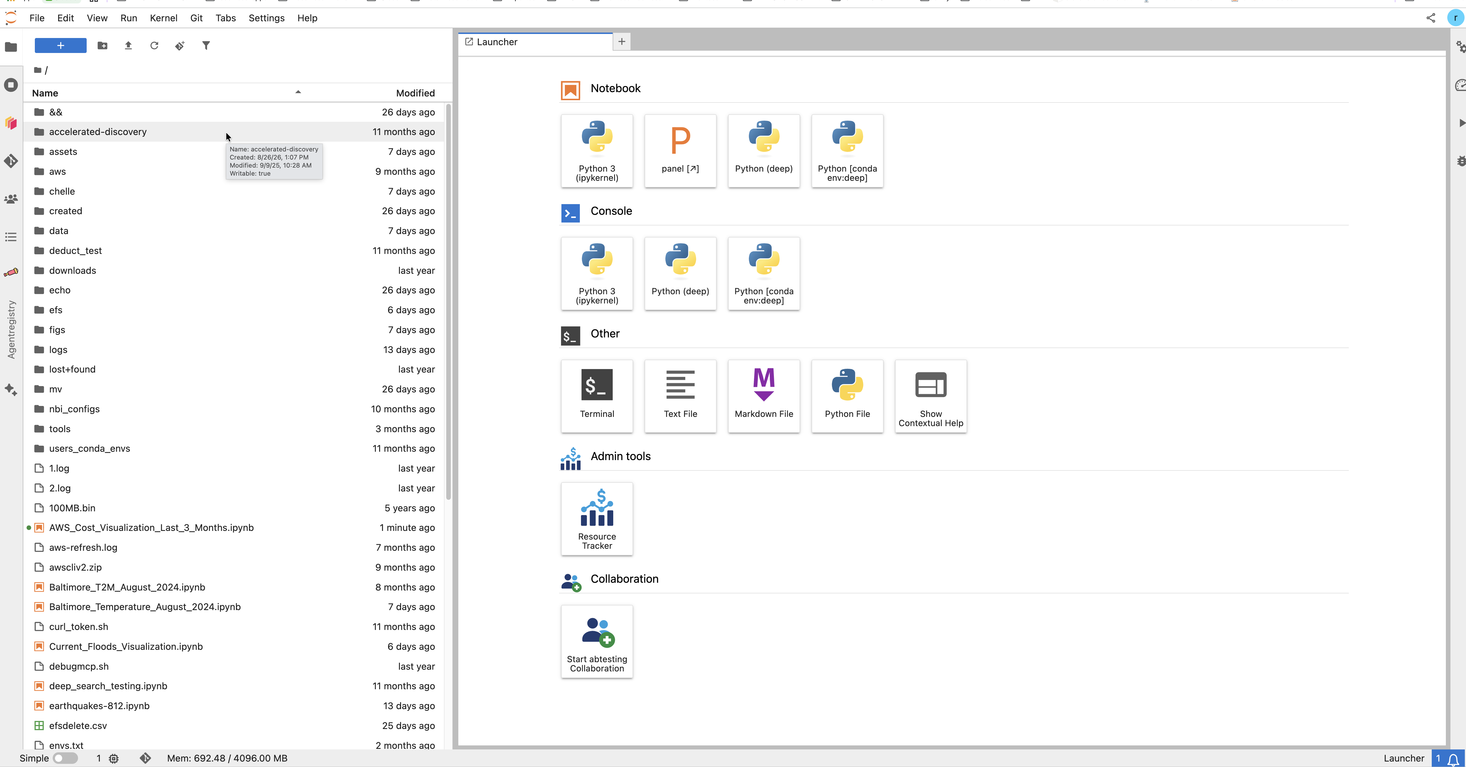
JupyterLab. The file browser is on the left; the Launcher tiles are in the middle.

Step 4: Know Where to Put Your Files and What Survives a Restart

This is the most important thing to learn on day one. Some places keep your files. Some do not.

The rule: keep your work in ~, in /efs/…, or in object storage. Everything else disappears when your workspace restarts.

How big is your home folder? It starts at 10 GB. It can be made larger — ask the platform team for the size you need. Keep it sensible: a very large home volume makes your workspace slower to start. Large data belongs in /efs/<project> or in object storage.

Two things worth knowing:

• EFS shows you every project you belong to. Open /efs/ and you see a folder for each one. You cannot open other people's folders — the permissions stop you.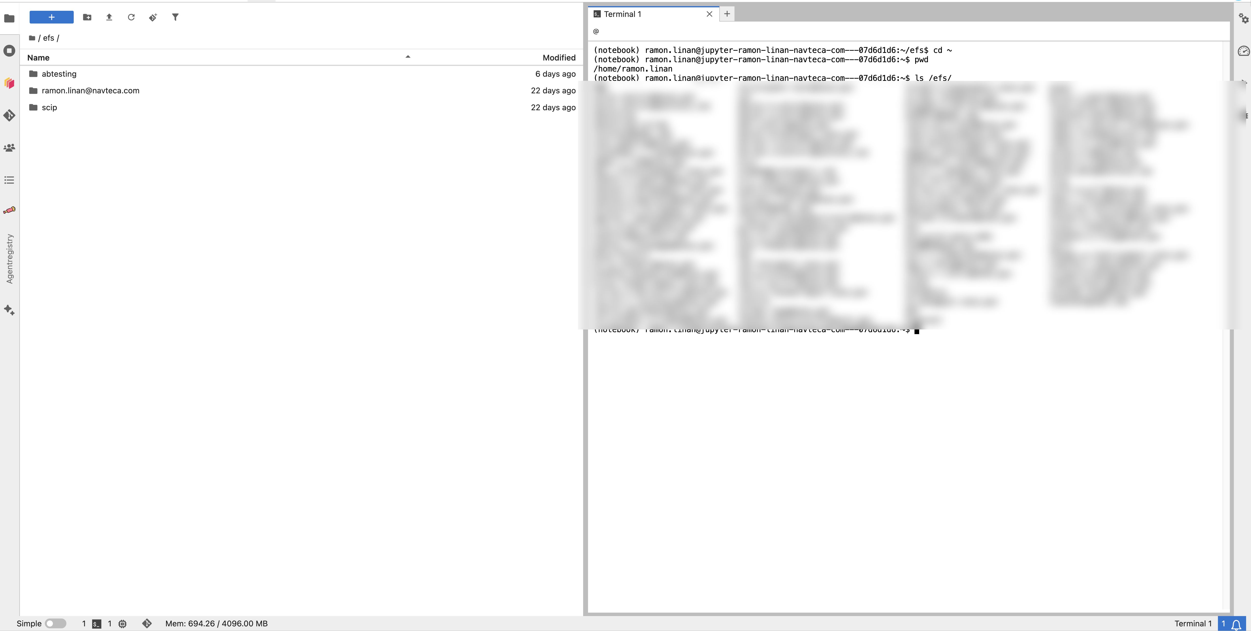
• The file browser and the terminal show the same files, laid out differently. The left-hand file browser and the command line have the same permissions. Do not worry if the two views look different.

The same files, two ways: the file browser on the left, a terminal on the right. The user list is blurred on purpose.

Which one should I use?

Step 5: Do the science

1. Open the Launcher and start a new notebook.
2. Type your code into a cell.
3. Press Shift + Enter to run it. The results will appear immediately below the cell.

Note: This behaves exactly like a standard Jupyter Notebook. If you've used Jupyter before, you'll feel right at home!

Step 5b: Create a Custom Kernel from a Conda Environment

Sometimes, the pre-configured software environments don't include the specific package versions your project requires. When this happens, you can build your own Conda environment and use it as a custom kernel.

• Environment: Your private, isolated set of software packages.
• Kernel: The computation engine that runs your code (this appears as an option in the notebook's "choose your language" menu).

Important: Always build your environment in your home folder. This ensures your custom packages persist and survive any system restarts.

1. To get started, open a Terminal from the Launcher and run the following commands:

# 1. create the environment (mamba is the fast version of conda)
mamba create -n myscience python=3.12 ipykernel -y

# 2. turn it on
conda activate myscience

# 3. add the packages you need
mamba install -c conda-forge xarray netcdf4 -y

That is all. The kernel appears in JupyterLab by itself, because the platform watches your environments for you.

1. Use Kernel → Change Kernel in your notebook and pick it.

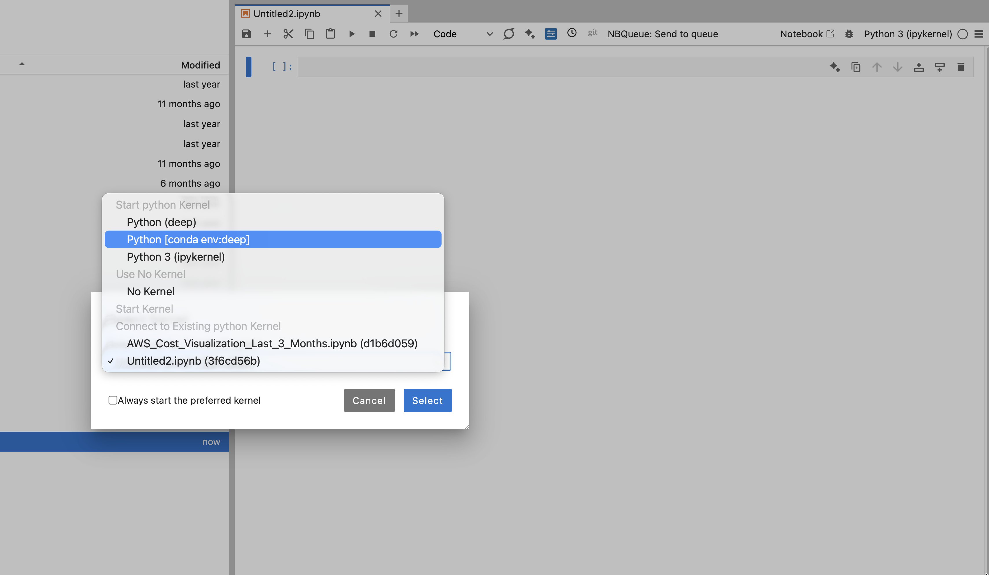
Kernel, then Change Kernel. Your own environment appears in the list.

Why this survives a restart: The platform is specifically set up to keep your environments safely tucked away in ~/users_conda_envs (inside your home folder). So, when you run mamba create -n myscience, it writes everything to /home/<your-username>/users_conda_envs/myscience. Because it's in your home folder, it'll be right there waiting for you tomorrow!

Two quick things to remember:

1. Always put ipykernel in the environment. If you forget this package, there won't be a kernel to pick from the notebook menu.
2. You can use conda or mamba. Both do the job, but mamba is much faster.

Kernel not showing up? If the kernel doesn't appear in your notebook menu, you can easily register it by hand. Just run this in your terminal: python -m ipykernel install --user --name myscience --display-name "My science env"

Step 6: Get SI Help While You Work

The Notebook Intelligence tool puts an SI assistant in JupyterLab.

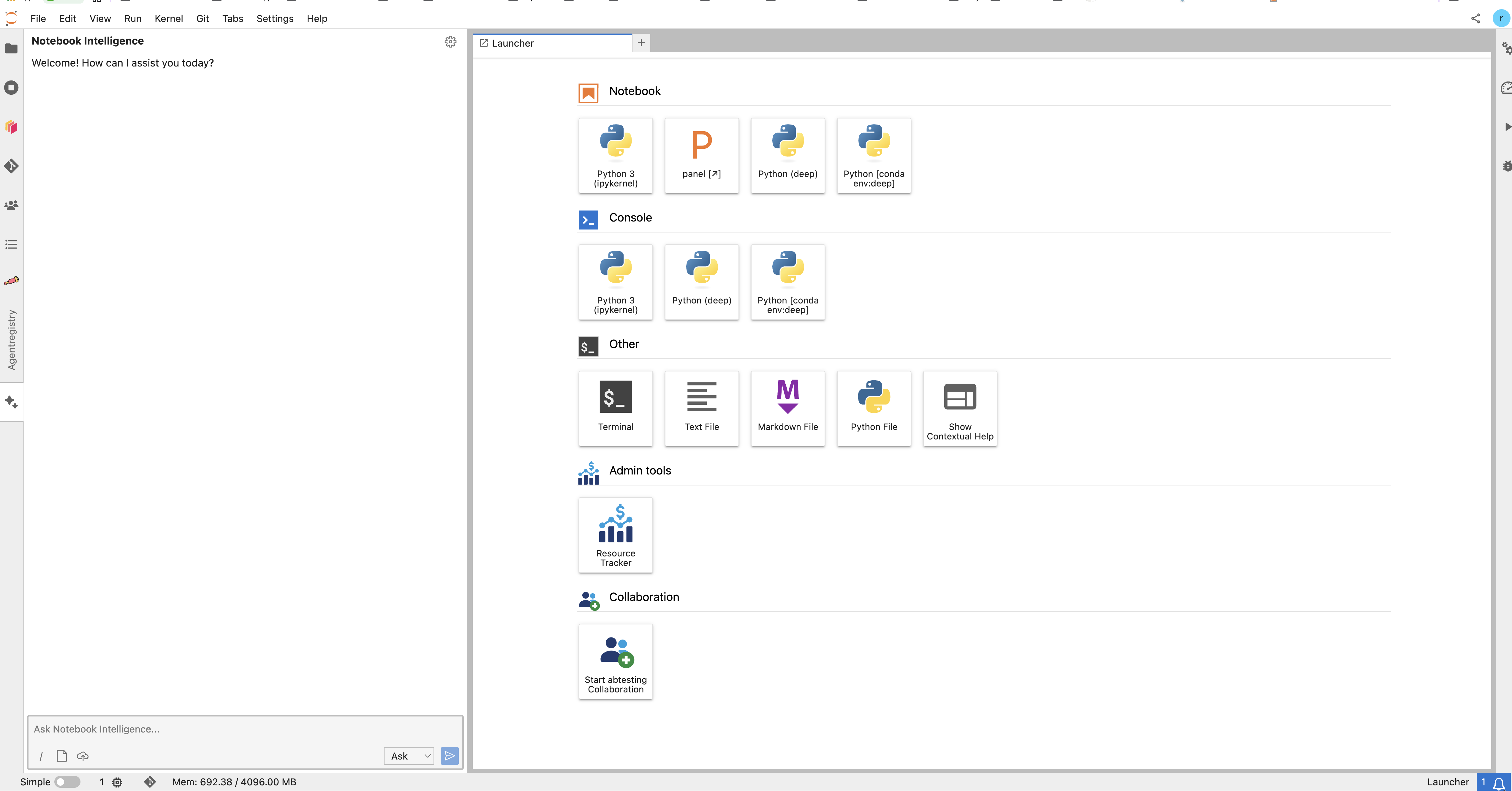
The Notebook Intelligence chat panel, open beside the Launcher.

You can also use your own model provider. See Notebook Intelligence and your LLMs.

Give the assistant new skills. The AgentRegistry panel in the left sidebar lists approved MCP servers — small services that teach the assistant a new trick, such as searching a data catalog. Press Add to NBI on one, and your assistant can use it. See the tool reference.

Step 7: Browse and Pull in Data

The data browser (jupyterlab-bxplorer) opens cloud storage inside JupyterLab. No command line needed.

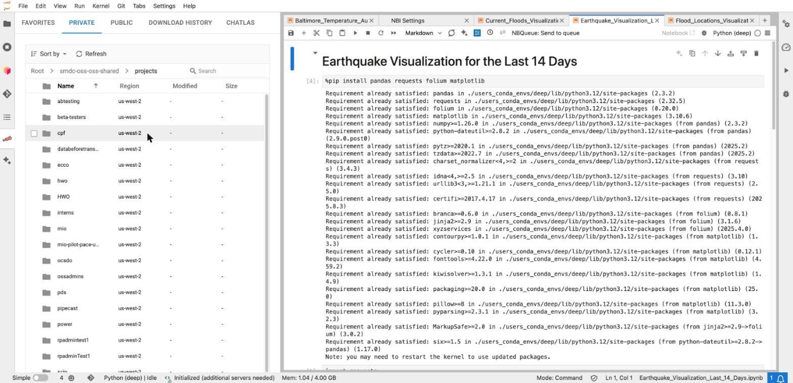
The data browser's PRIVATE tab: the platform bucket, opened to the shared projects folder.

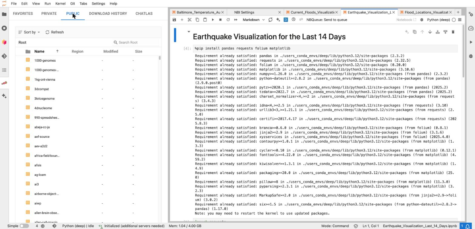
The data browser's PUBLIC tab lists public AWS science datasets.

Coming later: Google Cloud and Microsoft Azure storage.

Step 8: Need More Power? Two Choices

Choice A — many machines at once (Dask)

Use this when one analysis is too slow or too big for your workspace. Dask spreads the work over many machines and brings the answer back.

Start a cluster from your notebook, run the work, then shut the cluster down. The cluster costs money while it is up.

Choice B — send the job to the background (NBQueue)

Use this when a notebook takes a long time and you do not want to sit and watch it.

Open the notebook and press NBQueue: Send to queue in the toolbar at the top. Choose the machine, and send it. Then check the status in the NBQueue panel. When it finishes, the finished notebook, with its output, is waiting for you.

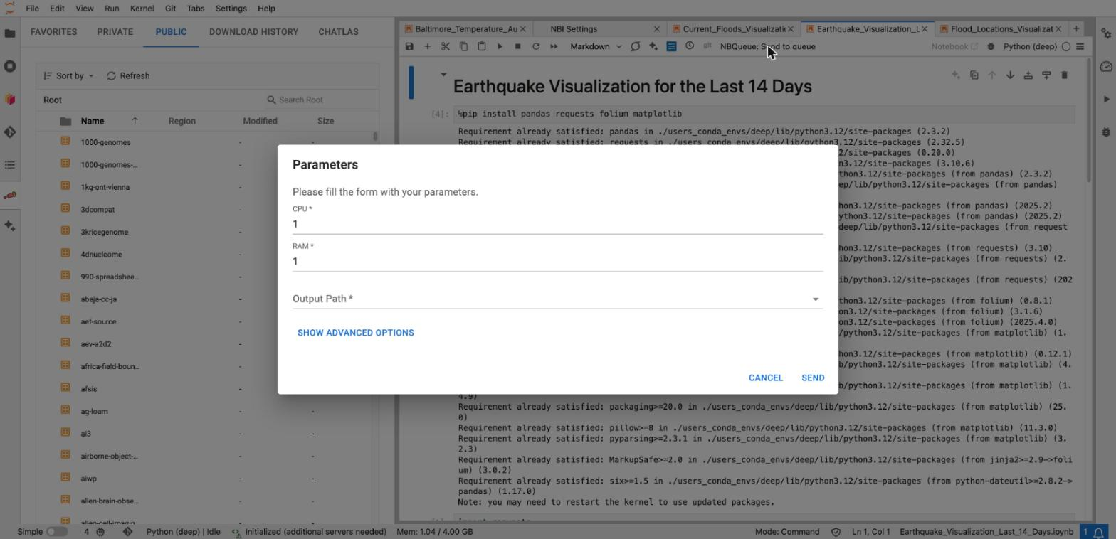
NBQueue asks for the CPU, the memory, and the output path. Then press SEND.

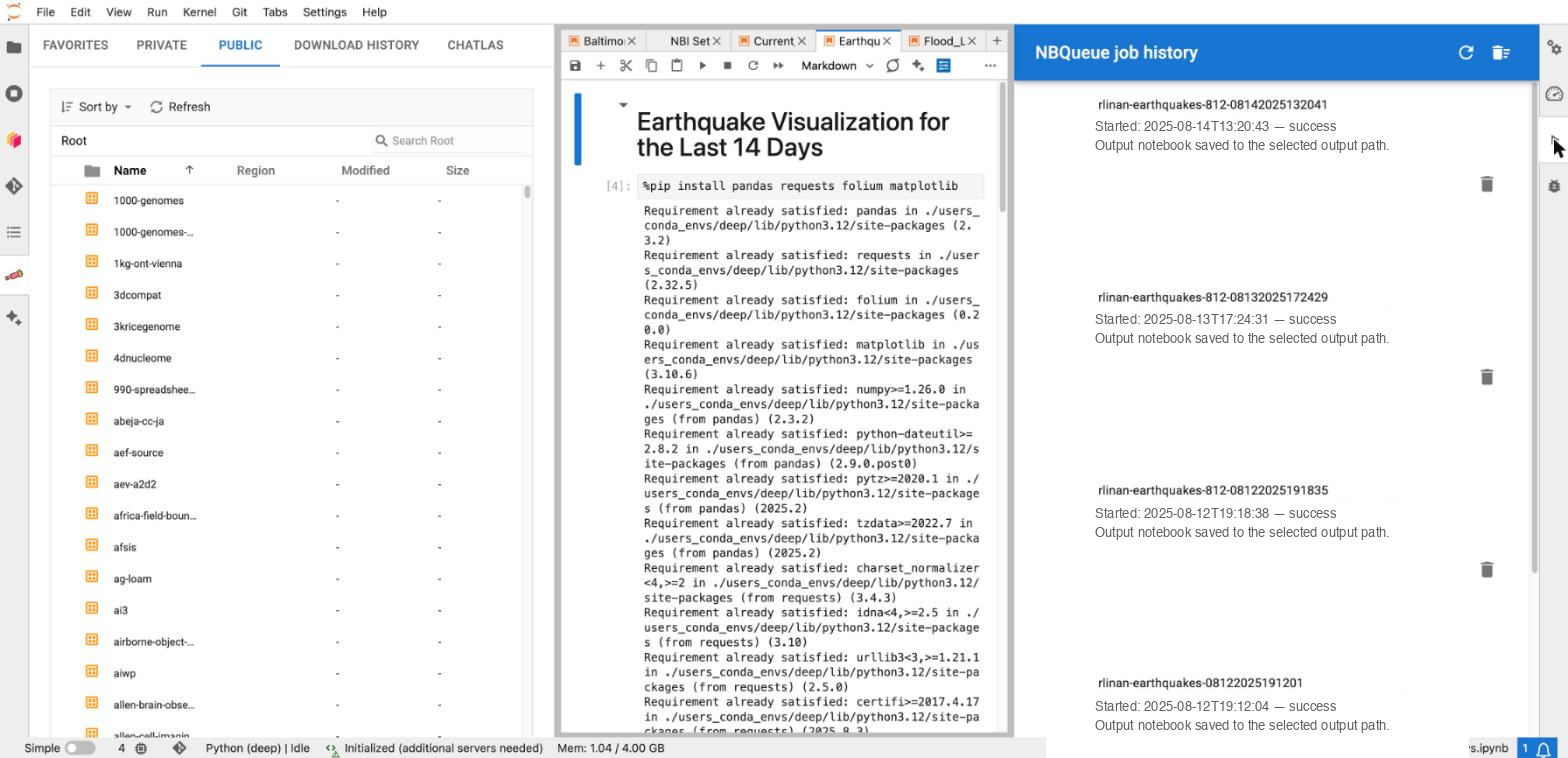
The NBQueue job history panel, in the right sidebar, lists your finished jobs.

Step 9: Work with Your Team on the Same File

If your project has collaboration turned on, your Launcher shows a Collaboration tile named "Start <project> Collaboration" — where <project> is the project you chose on the launch screen.

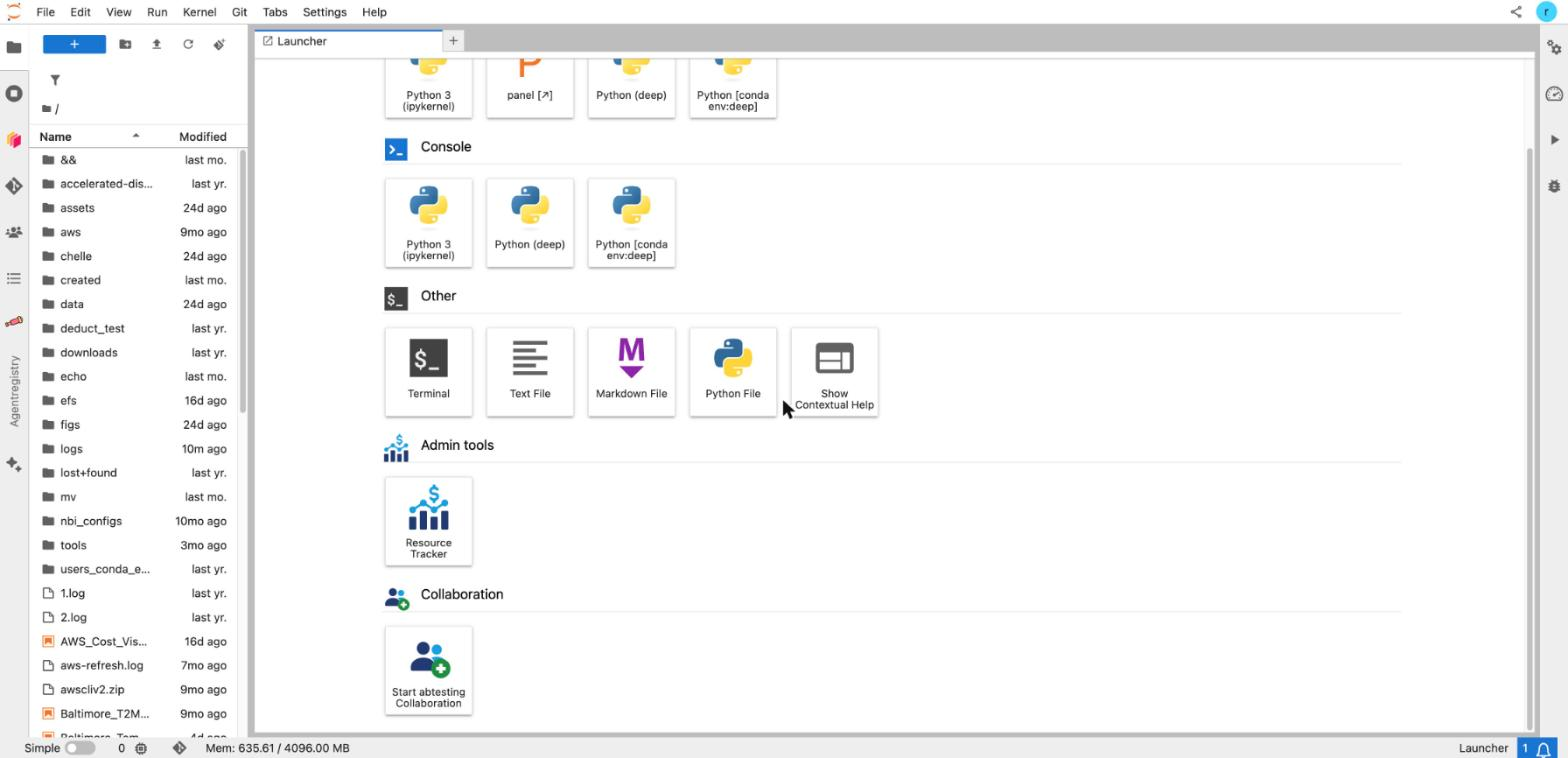
The Collaboration tile in the Launcher, before the shared session starts.

Save the group's work in /efs/<your project>. Files left in the shared session's own home folder can only be reached from inside that session.

When the work is done, click the tile again to stop the session. It costs the project money while it runs.

Full detail: Working together on the same notebook.

Step 10: Watch What You Are Spending

Open Resource Tracker — the tile under Admin tools in the Launcher. It shows:

• This month — hours used, compute cost, and storage cost split by type.
• Funding period to date — what you have used, what you were given, and what is left.
• When the numbers were last updated.

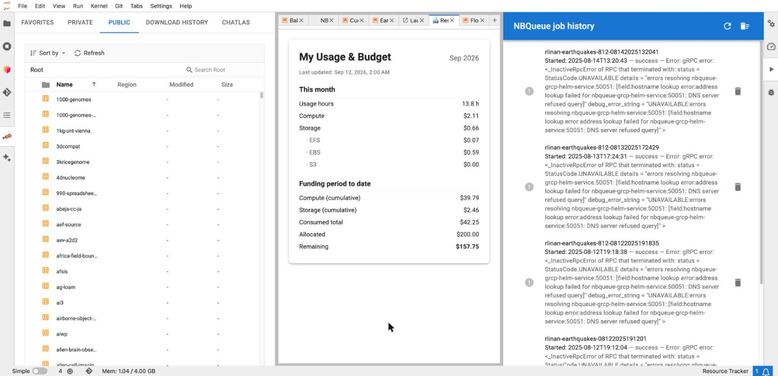
The Resource Tracker: This month, and Funding period to date.

Step 11: Stop When You Finish

This is the step people forget, and it is the one that costs money.

• Stop your notebook when you are done for the day.
• Shut down any Dask cluster.
• Stop the collaboration session when the group is finished.

Your files stay. Only the running machines stop. An idle session is closed automatically after about an hour, but do not rely on that — an open browser tab can keep it alive.

Where to get help

If you need help, contact support@sciencecloud.nasa.gov, or use the Science Cloud Support Portal.